Ways to demonstrate the CLT with purrr

The tidyverse is one of my favourite suites of R packages, and its idiomatic approach to data manipulation, analysis and visualization has heavily influenced how I approach data problems in R. If there’s one tidyverse package that best embodies these qualities, my vote is for purrr (opens in new tab)’s clean approach to iteration. purrr goes well beyond map and its variantsCheck out “purrr beyond map” (opens in new tab) for a great sampler., but it’s been far too easy to ignore anything beyond purrr’s simplest functions.

A while ago at work I had a great opportunity to dive deeper into purrr. While demonstrating the Central Limit Theorem to some colleagues, I whipped up a simulation of the dice-rolling experiment in R. I didn’t save the code, but it looked a lot like this:

library(tidyverse)
library(purrr)
library(rlang)

simulate_dice <- function(n, number_of_dice, ...) {
  seq.int(number_of_dice) %>%
    map(~sample(1:6, n, replace = T)) %>%
    as.data.frame(row.names = NULL) %>%
    rowwise() %>%
    summarize(average_of_dice = sum(c_across(where(is.numeric))) / {{number_of_dice}},
              number_of_dice = {{number_of_dice}})
}

clt_plotter <- function(df, x_value, facet_value) {
  df %>%
    ggplot() +
    geom_density(aes({{x_value}}, fill = "1"), colour = "black") +
    facet_wrap(vars({{facet_value}})) +
    guides(fill = F) +
    labs(x = "Sampling distribution of the mean",
          y = "Density")
}

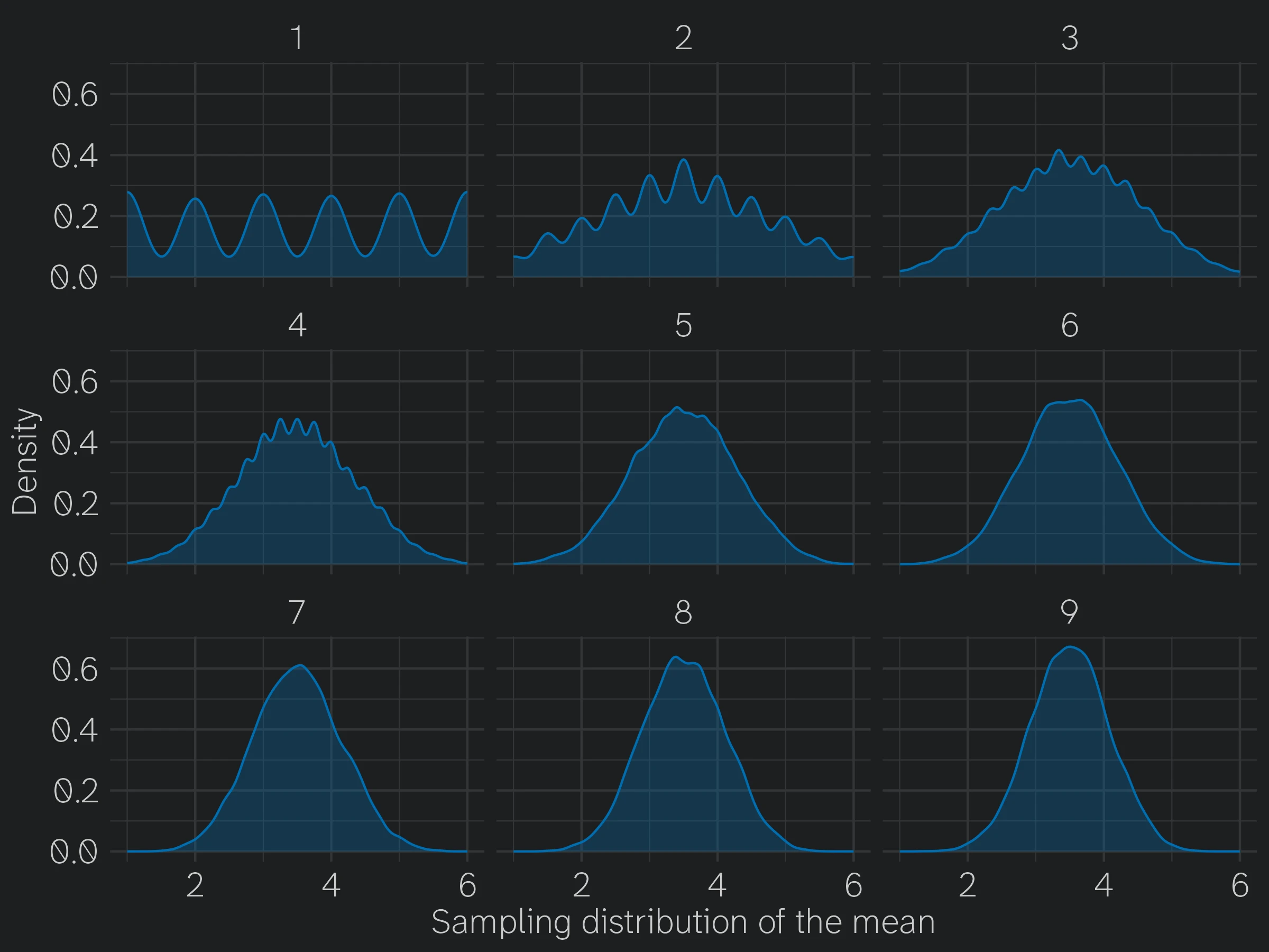
And here’s the output, after some styling. The wiggles in the number_of_dice = 1 facet are a necessary evil if we want to show the smooth behaviour for larger numbers of dice without customizing the density plots’ bandwidth and kernel.

set.seed(613)
1:9 %>%
  map_dfr(~simulate_dice(10000, .x)) %>%
  clt_plotter(., x_value = average_of_dice, facet_value = number_of_dice)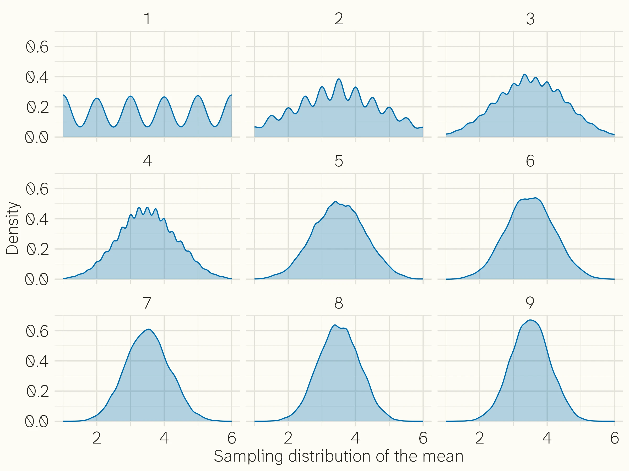

The simulate_dice code is functional but hacky:

• Heavy reliance on dataframes here is a problem, since we have to use the very slow rowwise operation to create a column containing the mean of each set of thrown dice.
• Inserting the number of dice thrown as its own column is an unappealing way to prepare clt_plotter for facetting.

We can improve this with purrr. We’ll start by writing a function that doesn’t immediately coerce everything to a dataframe. Instead, we’ll keep the results as a list as long as possible. To add the vectors element-wise, we can use purrr::reduce to avoid rowwise and mutate. Since addition is associative, we don’t need to specify the .dir argument for reduce.Originally I also wrote a division function, vector_division, to get the mean of each set of thrown dice, but it’s much faster to just divide the reduce by number_of_dice.

simulate_dice_list <- function(n, number_of_dice, ...) {
  seq.int(number_of_dice) %>%
    map(~sample(1:6, n, replace = TRUE)) %>%
    reduce(`+`) / number_of_dice
}

Now let’s compare the outputs to confirm that they’re identical. Since the new version doesn’t produce a dataframe, we’ll have to wrangle it into shape. enframe gives us a nested dataframe that requires unnest-ing. As we can see, the results are identical.

set.seed(613)
old_version <- 1:9 %>%
  map_dfr(~simulate_dice(10000, .x))

set.seed(613)
new_version <- 1:9 %>%
  map(~simulate_dice_list(10000, .x)) %>%
  enframe(.) %>%
  unnest(value)

identical(old_version$average_of_dice,
          new_version$value)

## [1] TRUE

So which is better? It all comes down to performance, which I assessed quickly with microbenchmark.

library(microbenchmark)

set.seed(613)
benchmark <- microbenchmark(
  `Original`    = 1:9 %>% map(~simulate_dice(1000, .x)),
  `New version` = 1:9 %>% map(~simulate_dice_list(1000, .x)),
  times = 50
)

summary(benchmark, unit = "ms")

## Unit: milliseconds
##         expr     min       lq     mean   median       uq    max neval
##     Original 1657.75 1673.737 1708.842 1689.758 1724.833 1904.5    50
##  New version    1.38    1.438    2.022    1.483    1.513   26.8    50

autoplot(benchmark) +
  scale_y_log10(labels = scales::comma)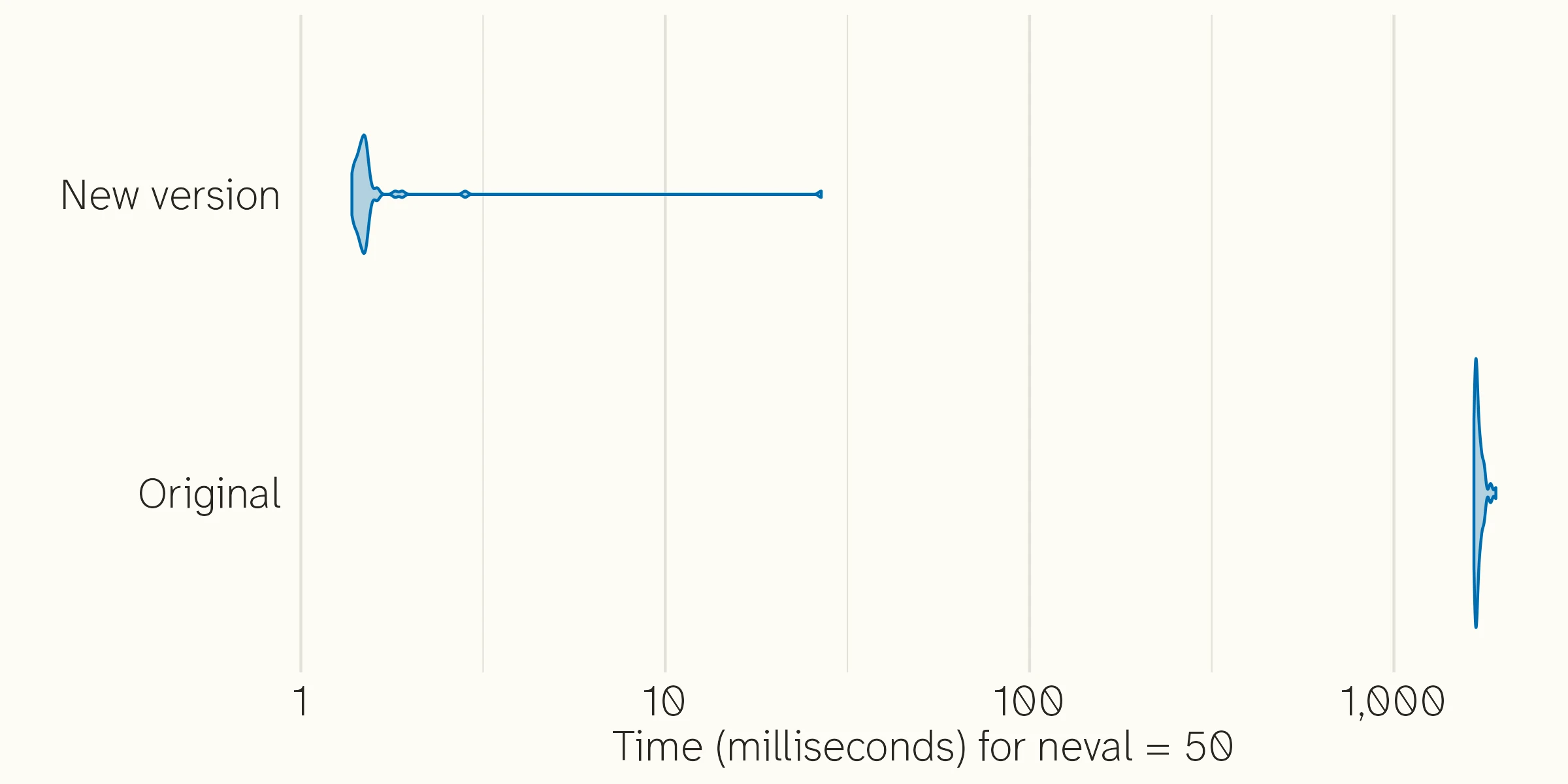

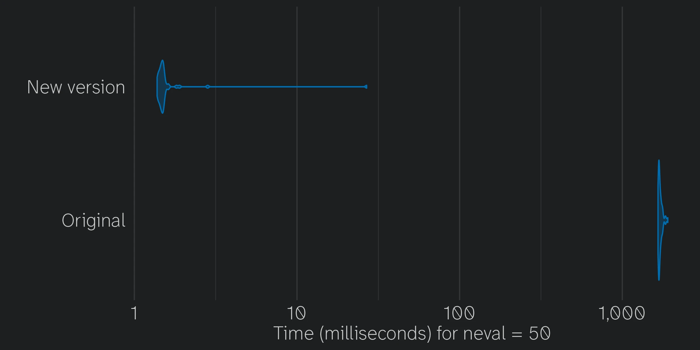
The difference is drastic: rowwise, while easy to pluck from the grab bag of dplyr tools, is indeed much slower than using lists.

Here’s the final code. As a bonus, we can avoid the summarize(number_of_dice = {{number_of_dice}}) code above by naming the input vector with setNames.

set.seed(613)
setNames(c(1:9), c(1:9)) %>%
  map(~simulate_dice_list(10000, .x)) %>%
  enframe(.) %>%
  unnest(value) %>%
  clt_plotter(., x_value = value, facet_value = name)

No difference in output, but faster and cleaner. It pays to use purrr in conjunction with more than just dataframes!